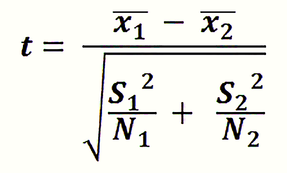
These differences are accounted for in the formula for Gosset's Student-t statistic:
where the difference in the sample means is in the numerator and the standard deviation of the difference in sample means in the denominator. Think about what happens in the formula depending on the size of the different values. For example, if the difference in the sample means is bigger, t is bigger because you are dividing into a larger number.
Student was the pen name that Gosset used. The formula is part of the statistics calculator below. The calculator is set up to compare the average weight of prospective NFL quarterbacks in 1987 and 2019. The resulting t = 5.51 tells us that the approximately 19 pound difference in the mean quarterback weights for the two years is 5.51 standard deviations above the average difference you would expect if the two groups were randomly broken into two groups and compared many, many times - like you did in the simulation.
t-Test Results
A t value of 5.51 is extremely unlikely. In fact, if you open the table indicating the 95% confidence level, you can see that any t value more than 2.145 standard deviations away from the mean difference would occur less than 5% of the time. Alternatively, t values less than or equal to 2.145 would occur 95% of the time. If the original hypothesis was that there was no difference in the weights, you can now say with 95% confidence that the hypothesis was wrong, that the average weights are significantly different.
Notice in using the table that the results depend on df, or the number of degrees of freedom in the comparison. The number of degrees of freedom indicates how many of the values are free to vary. In the case of a comparison of two groups like the one here the number of degrees of freedom is approximately one less than the smallest group size.
(Data can be changed in cells 3 and 4. q1 contains the list of earlier values; q2, the list of 2019 values.
The t value is found in cell 13.)
1) Compare running back weight for 1987 and 2019. If we originally assume that there is no difference in the two groups, what does the t value suggest about this hypothesis?
2) What if the sample sizes, the values of N, in the Student-t formula are bigger? Or, what if the variability, the values of S, in each sample are bigger or smaller? How is the value of t affected in these situations?
3) Are there significant differences between players at other positions from 1987 to 2019.
NFL combine statistics from NFL Combine Results. Downloaded August 29, 2019.
Desmos Graphing Calculator. (2015). Desmos Graphing Calculator. Accessed September 5, 2019].
